Possession of a ball in a ball game is a binary act. You either have it or you don’t. That means that the total value of stats associated with possession is also binary. This is true regardless whether the sport splits the value of a turnover in two or not, and notions of shared blame can cause issues when thinking about football. Football isn’t like other sports. Some of its “turnovers”, the punt especially, aren’t as easily quantifiable in the terms of other sports.
As an example of shared blame, we’ll take on the turnover in basketball. The potential value of the shot in the NBA is one point. This is easy to see, because a shot is worth 2 points and a typical NBA shooting percentage is about 50 percent (or a 3 point shot, with a percentage around 33%). That said, the value of the possession is two points, and the total value of the turnover is also two points.
Wait a minute, you say. The STL stat is generally only valued at 1 point. How can it be two? Well, there are two stats associated with a turnover in basketball. There is the TO stat, and the STL stat. And in metrics like the NBA Efficiency metric, each of these stats is valued at a point. TO + STL = total value of 2 points. The turnover in basketball is worth 2 points, and thus the possession is worth two points. The sum gets hidden because half of it is credited to the thief, and half is debited from the one who lost the ball.
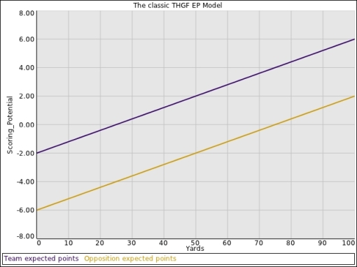
The classic description of the turnover in football derives from the Hidden Game of Football, and because their equivalent points metric is linear and independent of down and to go measures, the resultant value for the turnover is a constant. This isn’t easy to see in traditional visual depictions, but becomes easy to see when you flip the opposition values upside down.
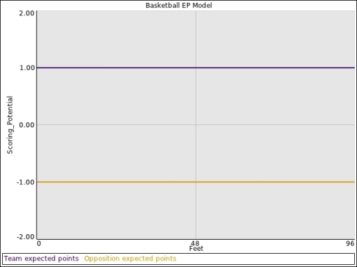
See how the relative distance between the lines never change? By the way, you can do the same thing for basketball, though the graph is a bit on the trivial side.
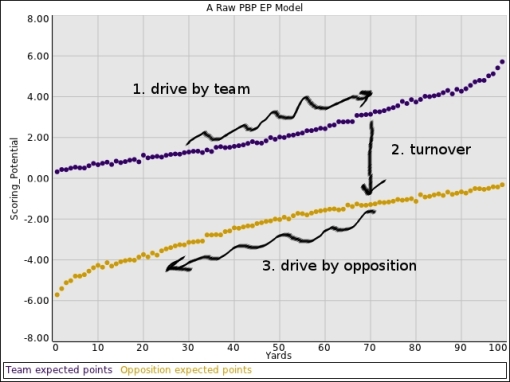
These twin plots are a valuable way to think about the game, turnovers, and for that matter, the game of football as a series of transitions between states. For now, by way of example, we’ll use these raw NEP data I calculated for my “states” post. We’ll plot an opposition set of data upside down and show what a state transition walk might look like using these data.
Not that complicated, is it? You could visualize these data two ways: as a kind of “Youtube video” where the specific value for the game changes as plays are executed, and the view remains 2D, or as a 3D stack of planes, each with one graph, each plane representing the game at a single play in the game.
Even in football, though, you could attempt to split the blame for the turnover into two parts: there is the person that lost the ball, and the person that recovers it. So the value for the state transition from one team to the next could be split in two, a la basketball, and credit give to the recovering side and a debit taken from the side losing the ball.
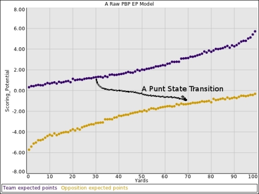
So what about the punt? It has no equivalent in basketball or baseball, and in general, looks just like a single state transition.
It’s a single whole, and therefore, you can get yourself into logical conundrums when you attempt to split the value of the punt in two.
This whole discussion, by the way, is something of an explanation for Benjamin Morris and folks like him, who saw his live blog on October 9, 2011. It’s not easy getting this point across using his graphics on his site. My point is more fully developed above, and why I was saying the things I did more evident from the graphics above.
Ben, btw, is an awesome analytics blogger. Please don’t take this discussion as any kind of indictment of his work, which is of a very high quality.


October 11, 2011 at 3:55 pm
Here’s the comment I posted in response on my blog. I have a longer post in the works that I’ll try to get up today or tomorrow:
Charitably, we may ultimately be arriving at (nearly) the same place via different routes, but barring that I think your analysis is making a big mistake.
Think of the game in terms of reciprocal possessions. Though turnovers may have specific effects on the expectation of your next drive (like when you get a turnover in your own territory), it doesn’t increase your expected number of possessions vs. theirs. It “fixes” the scoring potential of the last possession at 0, and then moves to the next iteration in the ongoing exchange.
For a “toy” game that illustrates the point, think of Baseball. When you get an out that ends your opponent’s inning, yes, you get to bat next—but that out isn’t worth the value of retiring the other team PLUS the value of batting: each team is going to get the same number of batting opportunities regardless.
This should be obvious for Baseball, but Football and Basketball are basically the same, except that the total number of opportunities in a game is variable. With the exception of fence-post possessions at the end of a half or game, the total number of possessions for each side will always be equal, no matter how many turnovers you get.
October 11, 2011 at 5:35 pm
Seems to me you have some ideas about possession reciprocity in mind, but they appear to me to be irrelevant to the issue at hand. And the issue is the best way to value a punt. I’m suggesting it should be treated as a single value, akin to a state transition in a state machine, or like electronic transitions in spectroscopy.
How hard is that?
And you need that notion to then go on and make decisions about the difference between a punt on 4th down and whether to go for it.
Because throwing all fancy words and language aside, that was the nature of our disagreement, how a punt should be valued in the context of a 4th and 1 decision.
And if my langauge is abstract, please blame Stuart Kaufmann, whose discussion of evolution as a Hamiltonian walk on a rugged landscape still speaks to the power of a good mathematical metaphor in a complex situation. I think the idea of a football game as a walk across a pair of net expected points curves is (for me at least) really evocative.
October 11, 2011 at 9:18 pm
I completely understand your “state transition” concept, I just happen to think it doesn’t accurately describe what’s going on.
The problem is that you’re not actually taking your opponent’s possesion away, you’re simply delaying it a little while. Again, with the exception of the minor effect keeping the ball will have on your winning the “fencepost possession”, and the effect your keeping the ball will have on the expectation of your opponent’s next possession (which, ideally, should be accounted for in your valuation metric), the only thing your conversion changes is the expectation of your current drive: from 0 to whatever.
I will work on formalizing this a bit better for my post on the subject, but for now, here’s another intuitive example: Imagine you successfully convert five 4th downs on a single drive, and end up kicking a field goal, what have you gained? By your “state transition” formulation, you would have gained the 3 points on your side of the ball, but also you’d be credited with denying your opponent 5 possessions! This is ludicrous: Assuming you used the same amount of clock time, your drive, in total, was actually worth *exactly* the same amount as if you had just marched down the field and kicked the FG.
Finally, I don’t mean for this to sound confrontational or dissmissive — I respect your blog and your work, I just happen to think you’re wrong on this point, and I apologize if I’m inarticulate in my responses (if anyone is having difficulty with abstract language, it’s me).
October 12, 2011 at 6:58 am
Ben,
I too am concerned this doesn’t spill over into incivility. I’ve seen talented men disagree with class, I’d love to keep it that way here.
In terms of the “value of the possession”, it only comes into play the moment you get the ball. Once you have the ball, the “value of the possession” is a bit like virginity. You can’t regain it, you can only lose it.
So, in the long drive description above, what the possession gets you is the ability to advance the ball or lose the ball (i.e. travel along your own EP curve). If you score, you score. And scoring potential (and yes, the allusion to a chemical potential is deliberate) isn’t the same as scoring.
Now, back to 4th and whatever and to put numbers to it..
A. 4th and 1, 70 yards to go
B. 1st and 10, 69 yards to go
C. Opponent’s 1st and 10, 70 yards to go.
D. Opponent’s 1st and 10, 30 yards to go.
Those are the states being compared, if your punter reliably gets 40 net yards per punt. And because states B, C, and D involve a possession, you have to take into account the value difference between the two.
Now the charts above mix all downs (really, only suitable for figuring out the reliability of older linear models IMO) and don’t answer those questions, which require far more specific EP curves. But the unsmoothed “raw” EP numbers I get out of my database are..
4th and 1, 70: 0.36
1st and 10, 69 : 1.53
1st and 10, 70 : 1.42
1st and 10, 30 : 3.31
If I do a quadratic fit to first and 10 data, I get fitted parameters that yield 1.48 and 1.52 respectively for 70 and 69. Take that for what it’s worth. But from this, we can now put numbers to an argument and see if we’re really all that far apart.
David.