Drawing a good diagram of a pass defense.

This is a follow up on my three part article, “Drawing a good diagram of a football field“. After trying for some time to automate arrow drawing, I’ve come to the conclusion that using GIMP, an arrow drawing plug-in, and GIMP’s path tool (a way to draw both straight lines and curves) are adequate to handle this problem.

Needed:

1. Diagram Drawing Tools (see my three part series here, here, and here).
2. A copy of GIMP. It’s free and available on Windows, Mac, and Linux.
3. Some experience with layers on GIMP. Start by searching “How to use layers in GIMP”. There are some nice Youtube videos that can get you started here.
4. This article is also really good: “How to Draw Arrows in Gimp”. Get the arrow plugin, install it, and read the instructions.
5. Look further at GIMP pathing with the search: “using path tool in gimp”.
6. For dashed and dotted lines, search using this phrase: “dashed lines in gimp”.

Some notes about drawing diagrams. If you’re using Windows shell to draw, then you’ll have no issues with Image::Magick. If you want to use the Perl interface to draw, then switch to Graphics::Magick, a fork of Image::Magick. Image::Magick has bugs when used with Perl.

When drawing arrows on a 640×480 diagram scaled in the way I’ve been scaling them, a length of wings setting of 15 and a brush width of 2 works well. This can be paired with path lengths of 5.0 pixels and will do nicely.

Tampa under front, Tampa 2 zone defense. Modeled on the diagram in Matt Bowen’s Tampa 2 article.

Tom Landry’s 4-3 Inside, showing a 1960s era strong side rotating zone, an early Cover 3. SAM and left cornerback jam before falling into zone.

Drawing a zone drop.

Load your diagram. Add a new transparent layer. Make sure you’re drawing on the transparent layer. Use the rectangle select tool (letter “R”). Choose a region to highlight as a zone. At this point select the bucket fill tool (shift B) and then select the color for the bucket fill. Use a foreground fill and set the opacity to about 50%. If your field is light green, use a dark green to fill the zone.

If you have more than one zone to add, add them all now.

Once complete, select all (important) and add another layer. On this new layer, add a path from the middle of the zone to the player. Select Tools -> Arrow (you added the arrow plugin, didn’t you?). Adjust arrow length of wings and brush width and draw the arrow. Repeat as needed.

If the path isn’t straight or you need a bar to create a “jam”, just use the path tool as needed.

If you want to add text or label the diagram, I’d suggest adding another transparent layer and putting the text above the main, zones, and arrows.

Once done, save the file as a GIMP native file and then again as a JPEG file. The second save will cause an export, crunching all the layers down to one image.

Miami 43, shade front, man plus cover 1 by the free safety.

Drawing man to man coverage

The trick here is to use the path tool to make a stippled (dotted) image. Choose a path from the defender to the player to be defended. When you choose stroke path, choose a line type (there are many). I like the stippled pattern, as it’s unlikely to be mistaken for a solid line.

 

Gillman and Coryell. Greatest versus Most Influential. Scoring Models are not obvious.

This is going to be a mixed bag of a post, talking about anything that has caught my eye over the past couple weeks. The first thing I’ll note is that on the recommendation of Tom Gower (you need his Twitter feed), I’ve read Josh Katzowitz’s book: Sid Gillman: Father of the Passing Game.

I didn’t know much about Gillman as a young man, though the 1963 AFL Championship was part of a greatest games collection I read through as a teen. The book isn’t a primer on Gillman’s ideas. Instead, it was more a discussion of his life, the issues he faced growing up (it’s clear Sid felt his Judaism affected his marketability as a coach in the college ranks). Not everyone gets the same chances in life, but Sid was a pretty tough guy, in his own right, and clearly the passion he felt for the sport drove him to a lot of personal success.

Worth the read. Be sure to read Tom Gower’s review as well, which is excellent.

ESPN is dealing with the football off season by slowly releasing a list of the “20 Greatest NFL Coaches” (NFL.com does its 100 best players, for much the same reason). I’m pretty sure neither Gillman nor Don Coryell will be on the list. The problem, of course, lies in the difference between the notions of “greatest” and “most influential”. The influence of both these men is undeniable. However, the greatest success for both these coaches has come has part of their respective coaching (and player) trees: Al Davis and Ara Parseghian come to mind when thinking about Gillman, with Don having a direct influence on coaches such as Joe Gibbs, and Ernie Zampese. John Madden was a product of both schools, and folks such as Norv Turner and Mike Martz are clear disciples of the Coryell way of doing things. It’s easy to go on and on here.

What’s harder to see is the separation (or fusion) of Gillman’s and Coryell’s respective coaching trees. Don never coached under or played for Gillman. And when I raised the question on Twitter, Josh Katzowitz responded with these tweets:

Josh Katzowitz : @smartfootball @FoodNSnellville From what I gathered, not much of a connection. Some of Don’s staff used to watch Gillman’s practices, tho.

Josh Katzowitz ‏: @FoodNSnellville @smartfootball Coryell was pretty adament that he didn’t take much from Gillman. Tom Bass, who coached for both, agreed.

Coaching clinics were popular then, and Sid Gillman appeared from Josh’s bio to be a popular clinic speaker. I’m sure these two mixed and heard each other speak. But Coryell had a powerful Southern California connection in Coach John McKay of USC, and I’m not sure how much Coryell and Gillman truly interacted.

Pro Football Weekly is going away, and Mike Tanier has a nice great article discussing the causes of the demise. In the middle of the discussion, a reader who called himself Richie took it upon himself to start trashing “The Hidden Game of Football” (which factors in because Bob Carroll, a coauthor of THGF, was also a contributor to PFW). Richie seems to think, among other things, that everything THGF discussed was “obvious” and that Bill James invented all of football analytics wholesale by inventing baseball analytics. It’s these kinds of assertions I really want to discuss.

I think the issue of baseball analytics encompassing the whole of football analytics can easily be dismissed by pointing out the solitary nature of baseball and its stats, their lack of entanglement issues, and the lack of a notion of field position, in the football sense of the term. Since baseball doesn’t have any such thing, any stat featuring any kind of relationship of field position to anything, or any stat derived from models of relationships of field position to anything, cannot have been created in a baseball world.

Sad to say, that’s almost any football stat of merit.

On the notion of obvious, THGF was the granddaddy of the scoring model for the average fan. I’d suggest that scoring models are certainly not obvious, or else every article I have with that tag would have been written up and dismissed years ago. What is not so obvious is that scoring models have a dual nature, akin to that of quantum mechanical objects, and the kinds of logic one needs to best understand scoring models parallels that of the kinds of things a chemistry major might encounter in his junior year of university, in a physical chemistry class (physicists might run into these issues sooner).

Scoring models have a dual nature. They are both deterministic and statistical/probabilistic at the same time.

They are deterministic in that for a typical down, distance, to go, and with a specific play by play data set, you can calculate the odds of scoring down to a hundredth of a point. They are statistical in that they represent the sum of dozens or hundreds of unique events, all compressed into a single measurement. When divorced from the parent data set, the kinds of logic you must use to analyze the meanings of the models, and formulas derived from those models, must take into account the statistical nature of the model involved.

It’s not easy. Most analysts turns models and formulas into something more concrete than they really are.

And this is just one component of the THGF contribution. I haven’t even mentioned the algebraic breakdown of the NFL passer rating they introduced, which dominates discussion of the rating to this day. It’s so influential that to a first approximation, no one can get past it.

Just tell me: how did you get from the formulas shown here to the THGF formula? And if you didn’t figure it out yourself, then how can you claim it is obvious?

 

Playoff Predictions, 2012 style

The three sites we noted last year: Cool Standings, Football Outsiders, and NFL Forecast, are at it again, providing predictions of who is going to be in the playoffs.

 

Cool Standings uses Pythagoreans to do their predictions (and for some reason in 2011, ignored home field advantage), FO uses their proprietary DVOA stats, and NFL Forecast uses Brian Burke’s predictive model.

Blogging the Beast has a terrific article on “the play”. If you watched any Dallas-Philadelphia games in 2011, you’ll know exactly what I mean, the way with a simple counter trap, LeSean McCoy treated the Cowboys line as if it were Swiss cheese.

Most important new link, perhaps, is a new Grantland article by Chris Brown of Smart Football. This article on Chip Kelly is really good. Not only is the writing good, but I love the photos:

Not my photo. This is from Chris Brown’s Chip Kelly article (see link in text).

as an example. Have you ever seen a better photo of the gap assignments of a defense?

 

Nascent 2012 analytics questions

After watching one or another controversy break out during the 2011 season, I’ve become convinced that the average “analytics guy” needs a source of play-by-play data on a weekly basis. I’m at a loss at the moment to recommend a perfect solution. I can see the play-by-play data on NFL.com, but I can’t download it. Worst case, you would think you could save the page and get to the data, but that doesn’t work. I suspect the use of AJAX or equivalent server side technology to write the data to the page after the HTML has been presented. Good for business, I’m sure, but not good for Joe Analytics Guy.

One possible source is now Pro Football Reference (PFR), which now has play by play data in their box scores, and has tended to present their data in AJAX free, user friendly fashion. Whether Joe Analytics Guy can do more than use those data personally, I doubt. PFR is purchasing their raw data from another source. And whatever restrictions the supplier puts on PFR’s data legally trickle down to us.

Further, along with the play by play, PFR is now calculating expected points (EP) along with the play by play data. Thing is, what expected point model is Pro Football Reference actually using? Unlike win probabilities, which have one interpretation per data set, EP models are a class of related models which can be quite different in value (discussed here, here, here). If you need independent verification, please note that Keith Goldner now has published 4 separate EP models (here and here), his old Markov Chain model, the new Markov Chain model, a response function model, and a model based on piecewise fits.

That’s question number one. Question that have to be answered to answer question one are things like:

• How is PFR scoring drives?
• What is their value for a touchdown?
• If PFR were to eliminate down and distance as variables, what curve do they end up with?

This last would define how well Pro Football Reference’s own EP model supports their own AYA formula. After all, that’s what a AYA formula is, a linearized approximation of a EP model where down and to go distance are ignored, with yards to score is the only independent variable.

Representative Pro Football Reference EP Values
1 yard to go		99 yards to go
Down	EP	Down	EP
1	6.97	1	-0.38
2	5.91	2	-0.78
3	5.17	3	-1.42
4	3.55	4	-2.49

 

My recommendation is that PFR clearly delineate their assumptions in the same glossary where they define their version of AYA. Make it a single click lookup, so Joe Analytics Guy knows what the darned formula actually means. Barring that, I’ve suggested to Neil Paine that they publish their EP model data separately from their play by play data. A blog post with 1st and ten, 2nd and ten, 3rd and ten curves would give those of us in the wild a fighting chance to figure out how PFR actually came by their numbers.

Update: the chart that features 99 yards to go clearly isn’t 1st and 99, 2nd and 99. Those are 1st and 10 values, 2nd and 10, etc at the team’s 1 yard line. The only 4th down value of 2011, 99 yards away, is a 4th and 13 play, so that’s what is reported above.

 

Tim Tebow, Eli Manning, and notions of clutchness

The fans were all nestled, all snug in their beds, while visions of clutch quarterbacks all danced in their heads.

Tim Tebow has managed to capture the imaginations of many announcers, fans, and analysts, including the eye of one Benjamin Morris. Ben posits, among other things,  that Tebow is being held back by his own conservatism,  that an inability to take passing risks in the first three quarters of the game is tossed aside in the fourth and some more true representation of his passing skill emerges.

This isn’t the first time that Ben has speculated on the nature of young quarterbacks and interceptions (This link is the most important, but also see here and here). One contradictory notion  that has come out of his analyses is that a lot of interceptions early in the career of a quarterback tends to be a good thing. It suggests a quarterback with exceptional skills testing those skills out — the idea that a talented cook has to get burned by his own grease to learn his chops spills over into the quarterbacking world.

A related question, important to NFC East fans, is Eli Manning clutch? This question was raised this year by Eli Manning’s exceptionally high ESPN QBR ratings relative to other metrics. People really got upset, claimed that the ESPN QBR was “busted”. But perhaps the ‘clutch’ factor actually saw something in Eli.

It’s almost a theme with the Giants that they fall behind and Eli either scores a couple late to win the game, or scores late to tie the game and then (win/lose) in overtime, or he puts on this furious rally that almost wins the game. They beat teams they shouldn’t, based on their Pythagoreans, and then lose to football patzers.

What to make of it? My gut unchecked feeling is yes, Eli is clutch, but  his team is another question altogether. It’s difficult to know with fans, emotions get the best of them. Donovan McNabb becomes Donovan McFlabb, good analysts try to prove that Jon Kitna is a better quarterback than Tony Romo, etc.

Thinking without benefit of numbers a bit further, Eli just doesn’t get ruffled. His play doesn’t suffer any effects of pressure. And that means, no matter how inadequate the team around him becomes, he’s still dangerous.

~~~

Kindle notes: just bought a Kindle Fire, and like it a great deal. It’s a better email platform than many web based email services, so it is  useful to forward  mails from those services to this device. I wish I could plug my  camera into the Kindle and upload photos, but  that will probably have to wait until Android 4 becomes a common base OS for these kinds of portable devices.

~~~~

Twitter notes: For those familiar with Smart Football, he tweets well, and is a useful feed if you’re at all interested. Trent Dilfer does quite a bit of good analysis via tweets. Surprisingly good is Doug Farrar, whose player analyses I tend to respect. I haven’t read much of Doug’s blog, Shutdown Corner, but given the character of his tweets, it might be worth a gander.

 

Playoff predictions and more, Thanksgiving 2011

There are three interesting sites doing the dirty job of forecasting playoff probabilities.  The first is Cool Standings, which is using Pythagorean expectations to calculate the odds of successive wins and losses, and thus, the likelihood of a team making it to the playoffs. The second is a page on the Football Outsiders’s site named DVOA Playoff Odds Report, which is using their signature DVOA stat – a “success” stat – to  generate the probability of a team making it to the playoffs. Then there is the site NFL Forecast, which has a page that predicts playoff winners using Brian Burke’s predictive model.

Of the three, Cool Standings is the most reliable in terms of updates. Whose model is actually most accurate is something any individual reader should try and take into consideration. Pythagoreans, in my opinion, are an underrated predictive stat. DVOA will tend to emphasize consistency and has large turnover penalties. BB’s metrics have tended to emphasize explosiveness, and now recently, running consistency, as determined by Brian’s version of the run success stat.

I’ve found these sites to be more reliable than local media (in particular Atlanta sports radio) in analyzing playoff possibilities. For a couple weeks now it’s been clear, for example, that Dallas pretty much has to win its division to have any playoff chances at all, while the Atlanta airwaves have been talking about how Atlanta’s wild card chances run through (among other teams) Dallas. Uh, no they don’t. These sites, my radio friends, are more clued in than you.

 

Analytics News, Early November 2011

The Stathead blog is now defunct and so, evidently, is the Pro Football Reference blog. I’m not too sure what “business decision” led to that action, but it does mean one of the more neutral and popular meeting grounds for football analytics folks is now gone. It also means that Joe Reader has even less of a chance of understanding any particular change in PFR. Chase Stuart of PFR is now posting on Chris Brown’s blog, Smart Football.

The author of the Armchair Analysis blog, Jeff Cross, has tweeted me telling me that a new play by play data set is available, which he says is larger than that of Brian Burke.

Early T formations, or not?

Currently the Wikipedia is claiming that Bernie Bierman of the University of Minnesota was a T formation aficionado

U Minnesota ran the T in the 1930s? Really?

I’ve been doing my best to confirm or deny that. I ordered a couple books..

No mention of Bernie's T in this book.

I've skimmed this book, and haven't seen any diagrams with the T or any long discussion of the T formation. There are a lot of unbalanced single wing diagrams, though.

I also wrote Coach Hugh Wyatt, who sent me two nice letters, both of which state that Coach Bierman was a true blue single wing guy. In his book, “Winning Football”, I have yet to find any mention of the T, and in Rick Moore’s “University of Minnesota Football Vault”, there is no mention of Bernie’s T either.

I suspect an overzealous Wikipedia editor had a hand in that one. Given that Bud Wilkinson was one of Bernie’s players, a biography of Bud Wilkinson could be checked to see if the T formation was really the University of Minnesota’s major weapon.

 

There is only one ball in football: thoughts on the punt.

Possession of a ball in a ball game is a binary act. You either have it or you don’t. That means that the total value of stats associated with possession is also binary. This is true regardless whether the sport splits the value of a turnover in two or not, and notions of shared blame can cause issues when thinking about football. Football isn’t like other sports. Some of its “turnovers”, the punt especially, aren’t as easily quantifiable in the terms of other sports.

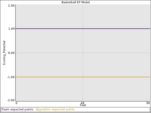
As an example of shared blame, we’ll take on the turnover in basketball. The potential value of the shot in the NBA is one point. This is easy to see, because a shot is worth 2 points and a typical NBA shooting percentage is about 50 percent (or a 3 point shot, with a percentage around 33%). That said, the value of the possession is two points, and  the total value of the turnover is also two points.

Wait a minute, you say. The STL stat is generally only valued at 1 point. How can it be two? Well, there are two stats associated with a turnover in basketball. There is the TO stat, and the STL stat. And in metrics like the NBA Efficiency metric, each of  these stats is valued at a point. TO + STL = total value of 2 points. The turnover in basketball is worth 2 points, and thus the possession is worth two points. The sum gets hidden because half of it is credited to the thief, and half is debited from the one who lost the ball.

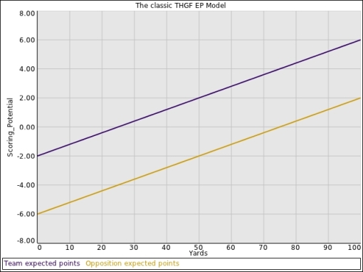
The value of the turnover is the difference in value between the curves.

The classic description of the turnover in football derives from  the Hidden Game of Football, and because their equivalent points metric is linear and independent of down and to go measures, the resultant value for the turnover is a constant. This isn’t easy to see in traditional visual depictions, but becomes easy to see when you flip the opposition values upside down.

See how the relative distance between the lines never change? By the way, you can do the same thing for basketball, though the graph is a bit on the trivial side.

This curve probably should have some distance dependence, actually.

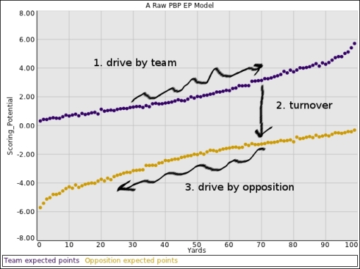
These twin plots are a valuable way to think about the game,  turnovers, and for that matter, the game of football as a series of transitions between states. For now, by way of example, we’ll use these raw NEP data I calculated for my “states” post. We’ll plot an opposition set of data upside down and show what a state transition walk might look like using these data.

The game of football can be described as a "walk" along a pair of EP curves.

Not that complicated, is it? You could visualize these data two ways: as a kind of “Youtube video” where the specific value for the game changes as plays are executed, and the view remains 2D, or as a 3D stack of planes, each with one graph, each plane representing the game at a single play in the game.

Even in football, though, you could attempt to split the blame for the turnover into two parts: there is the person that lost the ball, and the person that recovers it. So  the value for the state transition from one team to the  next could be split in two, a la basketball, and credit give to the recovering side and a debit taken from the side losing the ball.

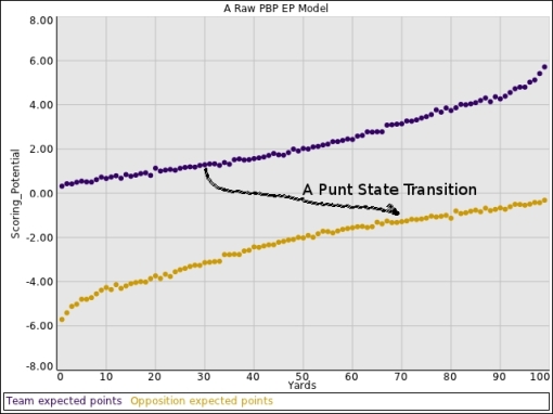
So what about  the punt? It has no equivalent in basketball or baseball, and in general, looks just like a single state transition.

The punt, in this depiction, is a single indivisible state transition from one team to the other.

It’s a single whole, and therefore, you can get yourself into logical conundrums when you attempt to split the value of the punt in two.

This whole discussion, by  the way, is something of an explanation for Benjamin Morris and folks like him, who saw his live blog on October 9, 2011. It’s not easy getting this point across using his graphics on his site. My point is more fully developed above, and why I was saying the things I did more evident from the graphics above.

Ben, btw, is an awesome analytics blogger. Please don’t take this discussion as any kind of indictment of his work, which is of a very high quality.

 

The NFL: on scoring and scoring potential

In chemistry, people will speak of the chemical potential of a reaction. That a mix of chemicals has a potential doesn’t mean the reaction will happen. There is an activation energy that prevents it. To note, the reaction energy can’t exceed the chemical potential of a reaction. Energy is conserved, and can neither be created nor destroyed.

Likewise, common models of the value of yardage assign a scoring potential to yards. I know of 5 models offhand, of which the simplest is the linear model (one discussed in The Hidden Game of Football). We’re going to derive this model by argument from first principles. There is also Keith Goldner’s Markov Chain model (see here and here), David Romer’s quadratic spline model (see here or just search for “David Romer football” via a good Internet search engine), the linear model of Football Outsiders in 2003, and Brian Burke’s expected points analysis (see here, here, here, and here). And just as in thermodynamics, where energy is conserved, this scoring potential has to be a conserved quantity, else the logic of the model falls apart.

One of the points of talking about the linear model is that is applies to all levels of football, not just the pros. Second, since it doesn’t require people to break down years worth of play by play data to understand it, the logic is useful as a first approximation. Third, I suspect some clever math geek could derive all the other models as Taylor series expansions where the first term in the Taylor series is the linear model itself. At one level, it has to be regarded as the foundation of all the scoring potential models.

Deriving the linear model.

If I start at the one yard line and then proceed back into my own end zone and get tackled, I’ve just lost 2 points. This is true regardless of the level of football being played. If instead I run 99 yards to my opponent’s end zone, I score 6 points instead. That means the scale of value in the common linear model is 8 points, and if we count each yard as equal in scoring potential, we start at -2 yards in my end zone, 6 in my opponents, and every 12.5 yards on the field, I gain 1 point of value. I do not have to crunch any numbers to assume this model as a first approximation.

Other models derive from analyzing a large data set of  games for down, distance, to go, and time situations.  They can follow all the consequences of being in  those down/distance combinations and  then derive real probabilities of scoring. We’re going to call those model EP, EPA or NEP models. The value in these models is rather than assuming some probability of scoring, average scoring probabilities are built into the model itself.

What’s the value of a turnover?

In the classic linear model,  as explained by The Hidden Game of Football, the cost of a turnover is 4 points. This is because the difference in value between both teams everywhere is 4 points.  The moment the model becomes nonlinear, that no longer applies. Both Keith Goldner’s model and the FO model predict that a turnover at the line of scrimmage minimizes in the middle of the field and maximize at the ends.

4 points is worth 50 yards. We’ll come  back to that in a bit.

What’s the value of a possession?

It’s the value of not turning  the ball over, and since we know the value of a turnover, in the linear model, possession is worth 4 points. In other models, this may change.

The value of the possession in  the linear model is always 4 points, even at the end of the game. To explain,  there are  two kinds of models that predict two kinds of things.

scoring potential models predict scoring

win probability models predict winning

The scoring potential of  the possession does not change as the game is ending. The winning potential does change and should change markedly as the game begins to end.

How much is a down worth?

This  is an important issue and not readily studied without a data heavy model. I’d suggest following a couple of the Brian Burke links above, they shed a terrific amount of light on the topic. Essentially, the value of a down at a particular time and distance is the difference in expected points at that time and distance between those downs.

How much is a touchdown worth?

We’ll start with the expected points models, because it becomes easy to see how they work. EPA or NEP style models have a total assigned value for the score (6.4 pts Romer, 6.3 Burke), so the value of scoring a touchdown is the value of the score minus the value of the position on the field. It has to be that way because the remaining value is a function of field position et al. If this isn’t true, you violate conservation of a scoring potential.

Likewise, in the linear model, the value of the touchdown is equivalent, due to linearity and scoring potential conservation, to the yards required to score the touchdown. This means if the defense recovers  the ball on the opponent’s 5  (i.e. the defense has just handed you 95 yards of value),  and your team runs for 3 yards, and then passes 2 yards for the score, that the value of the touchdown is 2 yards, or 0.16 points, and the value of the entire drive is 5 yards.

In this context, the classic interpretation of what THGF calls the new rating system doesn’t make a lot of sense.

RANKING = ( yards + 10*TDs – 45*Ints)/attempts

I say so because the yards already encompass the value of the touchdown(s). In this context, the second term could be regarded as an approximation of the value of the extra point (0.8 points of value in this case). And 45 instead of 50 is an estimation that the average INT changes field  position by about 5 yards.

Finally, this analysis begs the question of what model Pro Football Reference’s adjusted yards per attempt actually describes. I’ll try, however. If you adjust the value of yards to create a “barrier potential” term to describe the touchdown, you get the following bit of algebra

0.2(x + 2) + (x + 2 ) = value of true scoring difference = 6.4 + 2 = 8.4

1.2x + 2.4 = 8.4

1.2x = 6.0

x = 5

So, if you adjust the slope so the value of the line  at 100 equals 5 instead of 6, then the average value of a yard becomes 0.07 points, and the cost of  a turnover then becomes 3 points, or about 43 yards.

How much is a field goal worth?

The same logic that applies for a touchdown also applies for a field goal. It’s the value of the score minus the value of the particular field position, down, etc from which the goal is scored. Note that in a linear model, the value is actually negative for a field goal scored from the 37.5 yard line in. And  this actually makes sense, because the sum of the score values, as the number of scores grow large, in a well balanced EPA/NEP model should approach zero.  In the linear model, I suspect it will approach some nonzero number, which would be an approximation of  the average deviation from best fit EPA/NEP function itself.

Okay, so what if high scoring teams have this zero scoring value? What’s going on?

This is the numerator of a rate term, akin to that of a shooting percentage in the NBA. But since EP models are already averaged, the proper analogy is to the shooting percentage minus the league average shooting percentage. And to continue the analogy a bit further, to score in the NBA, you not only need to shoot (not necessary a good percentage), but you also need to make your own shot. Teams that put  themselves into position to score are the equivalent, they make their own shot. I’ll also note this +/- value probably also is a representation of the TD to FG ratio.

Conclusion

Scoring potential models are part of the new wave of football analysis and the granddaddy of all scoring potential models  is the linear model discussed extensively  in The Hidden Game of Football.  In these models, scoring potential is a conserved quantity and can neither be created nor destroyed. Some of the consequences of this conservation are discussed above.

 

Malcolm Gladwell’s “What the Dog Saw” and the fresh point of view

I’ve just started reading this book

and if only for the introduction, people  need to take a look at this book. This quote is pretty important to folks who want to understand how football analytics actually works, as opposed to what people tell you..

The other trick in finding ideas is figuring out the difference between power and knowledge. Of all the people whom you’ll meet in this  volume, very few of them are powerful or even famous. When I said I’m most  interested in minor geniuses, that’s what I mean.   You don’t start at the top if you want the story. You start in the middle, because the people in  the middle who do the actual work in the world….People at the top are self-conscious about what they say (and rightfully so) because they have position and  privilege to protect – and self-consciousness is the enemy of “interestingness”.

The more I read smaller blogs, the more I understand and the better I understand what I’m doing. To note, the Hidden Game of Football is also a worthwhile read, as those guys put a lot of effort into their work, into making it understandable, and a deeper read usually pays off in deeper understanding of concepts.

In Gladwell’s  book, there is a discussion of Nassim Taleb, currently a darling because of his contrarian views about randomness and its place in economics. But more immediately useful as a metaphor is Malcolm’s discussion of ketchup. He makes a strong case that the old ketchup formula endures because it’s hard to improve on.  It has just about  the right amounts of everything in the flavor spectrum to make it work for most people. I’m thinking the old NFL passer rating formula is much like that, though the form of  the equation is a little difficult for most people to absorb. I’ll be touching on ways to look at the passer rating in a much simplified form shortly.

Another story is in order here, the story of the sulfa drugs. To begin, recall that the late 19th century spawned a revolution in organic chemistry, which first manifested in new, colorful dyes. And not just clothing dyes, but also the art of tissue staining. The master of tissue staining back in the day was one Paul Ehrlich, who from his understanding of staining specific tissues, came up with  the notion of the “magic bullet”. In other words, find a stain that binds specifically to pathogens, attach a poison to the stain, and thereby selectively kill bacteria and other pathogens. His drug Salvarsan was the first modern antibacterial and his work set the stage for more sophisticated drugs.

Bayer found  the first of the new drugs, protonsil, by examining coal-tar dyes. However it only worked in live animals. A French team later found that in the body, the drug was cleaved into two parts, a medically inactive dye, and a medically active and colorless drug  that later became known as sulfanilamide. The dye portion of the magic bullet was unnecessary. Color wasn’t necessary to make the drug “stick”.

When dealing with formulas, you need to figure out ways to cut  the dye out of the equation, reduce formulas to their essence. Mark Bittman does that with recipes, and his Minimalist column in the Times is a delight to read. And  in football, needless complication just gets in the way. Figure it out, and then ruthlessly simplify it. And I suspect that’s the best path to  understanding why certain old formulas still have functional relevance in modern times.

Update: added link to new article. Fixed mixing of phrases silver bullet and magic bullet