In 1947, defensive theory in football had not yet advanced to the level of offensive theory. I’m saying this because the focus of defensive line play was gladitorial in nature: you would beat the man in front of you, pursue the ball carrier and tackle, preferably with the best form possible. Adjustments were rare. People had to accommodate man in motion but that was about it. The notion of a defensive key isn’t even talked about (1).
In the late 1940s to mid 1950s, defensive linemen were somewhat interchangable, and there were no specific guidelines for the sizes of defensive tackles, defensive ends, or middle guards. The roles of these linemen weren’t as detailed and specific as they are in modern days. There were big powerful immobile linemen, and smaller, faster, more nimble linemen. And though people like to think of linemen falling back into zones as a modern invention, the tactic was used in Steve Owen’s 6-1 Umbrella, and sees time in the pages of Dana Bible’s book:
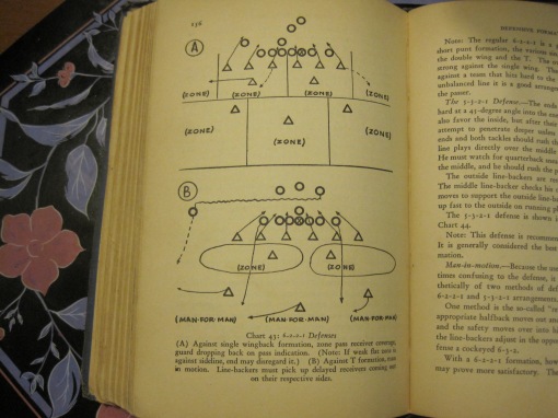
Linemen falling back and into coverage was a common tactic in 1947.
The idea, therefore, of a middle guard falling back into coverage wouldn’t have caused anyone in 1947 to blink an eye. So when you have a middle guard with sprinter’s speed, a guy like Bill Willis,
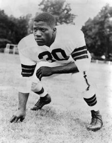
Cleveland Browns all pro middle guard Bill Willis (1946-1952). As big as the centers of his time with sprinter’s speed (2).
the idea that he should be a part of coverage would have been expected. Good linemen would fall back from the line and into coverage when the situation demanded. Linemen rushed yes, but behaved more like modern linebackers when they had to.
“He often played as a middle or noseguard on our five-man defensive line, but we began dropping him off the line of scrimmage a yard because his great speed and pursuit carried him to the point of attack before anyone would block him” (3)
So why is this important? It’s important because the dominant defensive front from 1950 or so through 1955 is a five man front, often a 5-2 Eagle. An example comes from this screen shot of video of the 1953 NFL championship
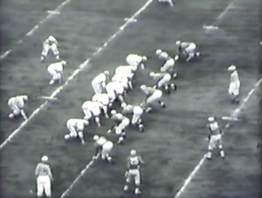
when diagrammed, would look something like this:
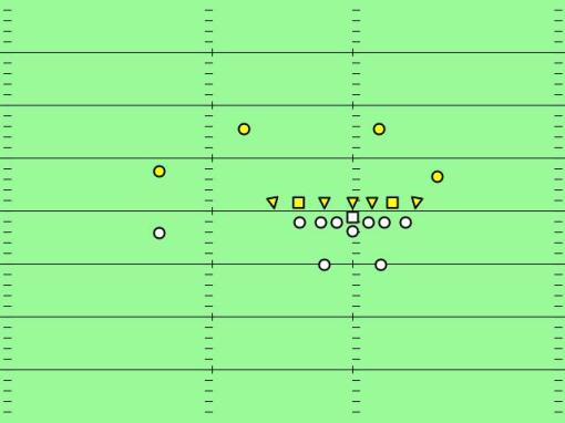
Typical five man front from early 1950s NFL football.
And therefore, the appearance of 4-3 fronts, as a product of a middle guard digging into the “bag of tricks” a lineman was supposed to know, should have been expected. 4-3s would have appeared as a poor man’s prevent defense, or as a response to specific game events, like quarterbacks throwing the ball just over the head of Chicago’s middle guard, Bill George.
…in a game against the Philadelphia Eagles, George made a now historic move that permanently changed defensive strategy in the National Football League.
On passing plays, George’s job was to bump the center and then drop back. George, noting the Eagles success at completing short passes just over his head, decided to skip the center bump and drop back immediately. Two plays later he caught the first of his 18 pro interceptions. While no one can swear which middle guard in a five-man line first dropped back to play middle linebacker and create the classic 4-3 defense, George is the most popular choice.
This game dates to 1954. Andy Piascik’s book claims that in the regular season game between the Detroit Lions and Cleveland Browns in 1952, the Lions employed a 4-3 (4). I’d suggest though, in the absence of any evidence to the contrary, that these 4-3s fall into the form of an adjustment to the 5-2, as opposed to an integral coordinated defensive system.
The deal is, by 1956, Tom Landry, as the defensive coordinator of the New York Giants, has a 4-3 that isn’t anyone’s adjustment to something else. It’s a full blown base defense, a creation of his own hard work and imagination. It’s a largely 1 gap, keying defense, with distinct assignments to the linemen. Linemen have to fill gaps and keep the offensive line from getting to the middle linebacker. The middle linebacker roams, tackles, covers his two gaps. The initial Landry defenses have been lavishly detailed in the two volume text “Vince Lombardi on Football“, because these were the defenses Vince took with him to Green Bay.
And while what video I can watch in the period from 1948 to 1955 has yet to yield a single 4-3, the Giants live in it in the 1956 Championship game, and after some initial five man line in the 1957 Championship game, Detroit soon switches to a 4-3 and stays in it.
All this lends credence to the words of Paul Zimmerman (5)
Here and there the 4-3 popped up around the league. The Eagles got into a form of it when they had their middle guard, Bucko Kilroy, stand up, though at 258 pounds he hardly had true middle-linebacker responsibilities. The Redskins tried it, lifting middle guard Ron Marcinak and substituting a linebacker, Charley Drazenovich.
Landry graduated from player to player-coach to defensive coach under Jim Lee Howell. Vince Lombardi ran the offense. In 1956 the Giants drafted a tackle from West Virginia, Robert Lee Huff, nicknamed Sam, who had been born to play middle linebacker in the 4-3, and that became the Giant’s official standard defense. By 1957 everyone was in it.
So the real question is, how much of this 4-3 defensive system was prior art? Not the positions, mind you, but the components. The keys, the coordination, the pieces? I think the minimum you need to make such a defense are these three elements.
1. Film study. Without it you can’t really predict trends.
2. Two platoon football. Otherwise, you’re teaching one player offense 80% of the time.
3. A modern coaching staff, with full time assistants.
It’s very clear that Paul Brown’s staff with the Cleveland Browns has these three elements in the 1950s, but I don’t see signs that they were unusually innovative on defense. Instead, what you see are things like references to three man single safety backfields (6), and signs that they were working within the status quo of the times.
One resource I’d love to get my hands on is the writings of the former Cleveland Browns linebacker, Hal Herring (7). He played for the Browns for three years, starting in 1950. Later, he wrote a dissertation that was titled “Defensive Tactics and Techniques in Professional Football.” I’m not close enough to a research library to know if it can easily be obtained, but back in the day when I was writing my own dissertation, we had to make dissertations available to just about anyone who wanted a copy.
Update: correction on the Bill George date.
~~~
Notes and References
(1) Keys and tells are different beasts. A tell is Dan Fouts giving away run or pass in 1979 with his feet placement. An example of a key is a person whose actions tell you where to go and what role to play when you do. Tells have been part of football forever, akin to stealing signs. Keys are elements of the game that have to be built into the defense and coached.
(2) Image from Special Collections, Cleveland State University Library.
(3) Paul Brown, quoted by Goldstein.
(4) Piascik, Chapter 11. The exact quote is:
“I think the 4-3 defense originated with him [Parker] and his coaches,” Dub Jones said of the Detroit team that so stifled Cleveland in that first ever meeting between the two teams. “They threw that in our face in ’52 and it was tough for us to cope with, having not faced it.”
(5) Zimmerman, Chapter 6.
(6) Brown and Clary, p 220, has this interesting blurb regarding the 1951 NFL championship:
For several years, our secondary had never declared a strong side of our opponent’s offensive formation until it saw which direction the fullback was going, and though we had gotten by with this strategy, it put a great burden on Cliff Lewis, the middle safety in our three-man secondary.
(7) Piascik, Chapter 8.
Bibliography
Bible, Dana X, “Championship Football”, Prentice-Hall, New York, 1947.
Brown, Paul and Clary, Andy, PB: The Paul Brown Story , Atheneum, New York, 1979.
Goldstein, Richard, “Bill Willis, 86, Racial Pioneer in Pro Football, Dies”, New York Times, Nov. 29, 2007, accessed Jun 7, 2013.
Piascik, Andy, The Best Show in Football: The 1946-1955 Cleveland Browns – Pro Football’s Greatest Dynasty [ebook]
Zimmerman, Paul, New Thinking Man’s Guide to Professional Football , Harper Collins, 1984.


